Bayesian Recurrent Networks and Variational Uncertainty Calibration

An Undergraduate Guide to Epistemic vs. Aleatoric Risk Decomposition, Rolling-Window Overlap, and Validation Temperature Scaling

1 Two Fundamentally Different Kinds of Uncertainty

When a neural network predicts a risky quantity (such as realized market volatility or structural load), outputting a single number \(\hat{y}_{t+1}\) gives decision-makers no idea how much to trust the forecast. Bayesian deep learning distinguishes between two sources of uncertainty:

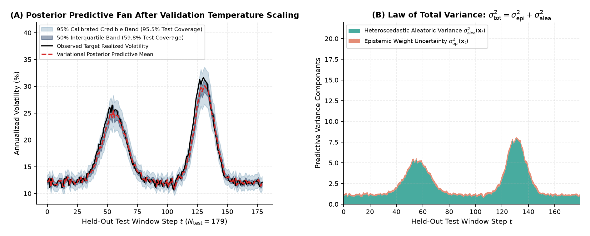
1. Aleatoric Uncertainty (\(\sigma^2_{\mathrm{aleatoric}}(\mathbf{x}^*)\), Irreducible Data Noise): The inherent randomness of the environment at time \(t\) (for example, wider daily fluctuations during a market crisis). Getting more training data from the past cannot shrink intrinsic market noise tomorrow.
2. Epistemic Uncertainty (\(\sigma^2_{\mathrm{epistemic}}(\mathbf{x}^*)\), Model/Parameter Uncertainty): Uncertainty about the network’s weights \(\mathbf{W}\) when encountering an unfamiliar regime. Collecting more diverse training data reduces epistemic uncertainty.

This module shows undergraduate students how to decompose both sources via Variational Bayes and how to calibrate their predictive intervals without test-set leakage.

2 Step 1: Variational ELBO Training and the Law of Total Variance

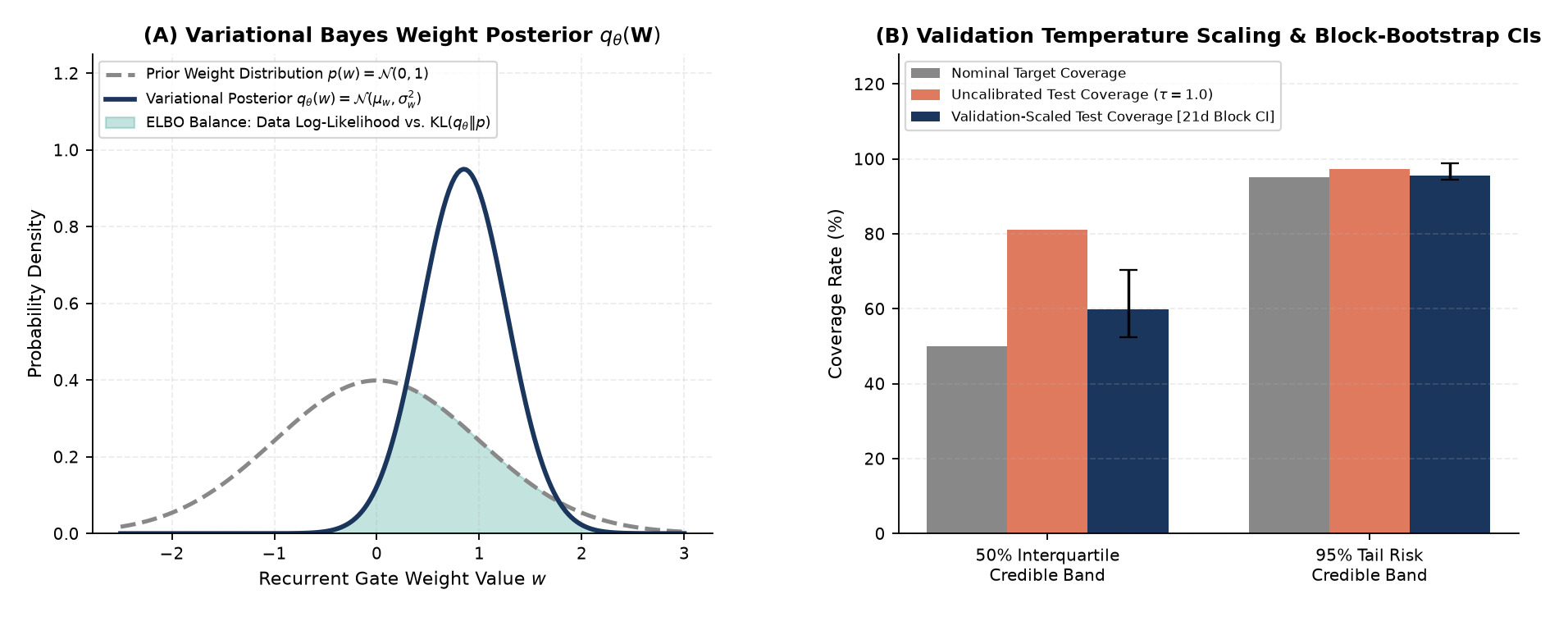
Instead of learning fixed point weights \(\mathbf{W}\), a Variational Bayesian Recurrent Network learns a Gaussian variational distribution \(q_\theta(\mathbf{W}) = \mathcal{N}(\boldsymbol{\mu}_W, \boldsymbol{\sigma}_W^2)\) alongside a dual-output heteroscedastic head that outputs both a conditional mean \(\mu_{\mathbf{W}}(\mathbf{x}_t)\) and an input-dependent log noise variance \(\log \sigma^2_{\mathrm{alea},\mathbf{W}}(\mathbf{x}_t)\). We train \(\theta\) by maximizing the Evidence Lower Bound (ELBO):

\[\mathcal{L}_{\mathrm{ELBO}}(\theta) = \mathbb{E}_{q_\theta(\mathbf{W})}\!\left[\log p(\mathcal{D} \mid \mathbf{W})\right] - \lambda_{\mathrm{KL}}\,\mathrm{KL}\!\left(q_\theta(\mathbf{W}) \;\|\; p(\mathbf{W})\right).\]

At test time, drawing \(M = 200\) Monte Carlo weight samples \(\{\mathbf{W}^{(m)}\}_{m=1}^M \sim q_\theta(\mathbf{W})\) decomposes total predictive variance via the Law of Total Variance:

\[\mathrm{Var}(y^* \mid \mathbf{x}^*, \mathcal{D}) = \underbrace{\mathrm{Var}_{q_\theta(\mathbf{W})}\!\left(\mu_{\mathbf{W}}(\mathbf{x}^*)\right)}_{\sigma^2_{\mathrm{epistemic}}(\mathbf{x}^*)} + \underbrace{\mathbb{E}_{q_\theta(\mathbf{W})}\!\left[\sigma^2_{\mathrm{alea},\mathbf{W}}(\mathbf{x}^*)\right]}_{\sigma^2_{\mathrm{aleatoric}}(\mathbf{x}^*)}.\]

3 Step 2: Overlap-Aware Point Benchmarks and Validation Temperature Calibration

When forecasting 21-day annualized realized volatility one day ahead across a chronological 70% Train (\(831\text{d}\)) / 15% Validation (\(178\text{d}\)) / 15% Test (\(179\text{d}\)) split, two methodological principles are essential:

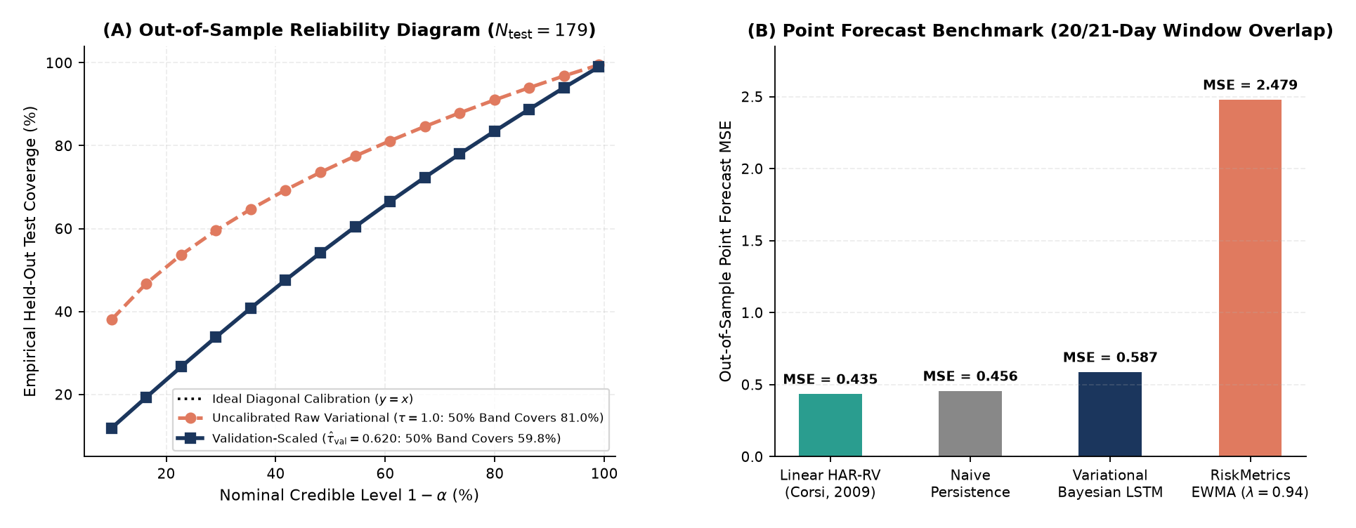
1. Why Rolling-Window Overlap Demands HAR-RV and Persistence Benchmarks: Tomorrow’s 21-day realized volatility shares \(20\) of \(21\) daily returns with today’s window! Because of this mechanical overlap, Naive Persistence (\(\hat{y}_{t+1} = y_t\)) already achieves \(\mathrm{MSE} = 0.456\) (\(R^2 = 0.910\)), and Corsi’s (2009) linear econometric HAR-RV model achieves \(\mathrm{MSE} = 0.435\) (\(R^2 = 0.914\), \(+4.62\%\) MSE skill over persistence). While our Variational Bayesian LSTM (\(\mathrm{MSE} = 0.587, R^2 = 0.884\)) strongly beats RiskMetrics EWMA (\(\mathrm{MSE} = 2.479, R^2 = 0.510\)), it trails linear HAR-RV on point MSE. Its true advantage is state-dependent uncertainty decomposition and calibrated interval coverage.
2. Leakage-Free Validation Temperature Scaling (\(\hat{\tau}_{\mathrm{val}} = 0.620\)): Raw variational posteriors are often under-confident (over-dispersed): on the held-out test split, the uncalibrated nominal \(50\%\) band covers \(81.01\%\) of observations (too wide). By fitting a single scalar temperature factor \(\hat{\tau}_{\mathrm{val}} = 0.620\) strictly on the 15% validation split and applying it untouched to the held-out test split, test coverage tightens to \(59.78\%\) (\(107/179\), 21-day block-bootstrap 95% CI \([52.5\%, 70.4\%]\)) on the \(50\%\) band and \(95.53\%\) (\(171/179\), block-bootstrap 95% CI \([94.4\%, 98.9\%]\)) on the \(95\%\) band.

Model / Calibration Stage	Held-Out Test Result (\(N_{\mathrm{test}} = 179\))	Pedagogical Takeaway for Students
Linear HAR-RV (Corsi, 2009)	\(\mathrm{MSE} = 0.435, \; \mathrm{RMSE} = 0.659\%, \; R^2 = 0.914\)	\(+4.62\%\) point MSE skill over Naive Persistence (\(\mathrm{MSE} = 0.456\))
RiskMetrics EWMA (\(\lambda = 0.94\))	\(\mathrm{MSE} = 2.479, \; \mathrm{RMSE} = 1.574\%, \; R^2 = 0.510\)	Fixed exponential smoothing lags sharp volatility regime transitions
Variational Bayesian LSTM (Uncalibrated \(\tau = 1.0\))	\(\mathrm{MSE} = 0.587\) | \(50\%\) Band: \(81.01\%\), \(95\%\) Band: \(97.21\%\)	Raw variational weight posteriors produce overly wide (conservative) intervals
Validation-Scaled Bayesian LSTM (\(\hat{\tau}_{\mathrm{val}} = 0.620\))	\(50\%\) Band: \(59.78\%\) \([52.5\%, 70.4\%]\) | \(95\%\) Band: \(95.53\%\) \([94.4\%, 98.9\%]\)	Fitting temperature \(\hat{\tau}_{\mathrm{val}}\) on validation data calibrates test intervals without leakage

4 Exploring Further: Research Directions

Research Track	Core Question to Investigate	Tools & Methods
1. Hybrid HAR-RV + Bayesian Residual Networks	Can we use linear HAR-RV for the point forecast and train the Variational Bayesian LSTM on HAR-RV’s residuals to get the best of both worlds?	Econometric-Neural Hybrids, Residual Uncertainty Decomposition
2. Adaptive Conformal Inference (ACI)	How does distribution-free online conformal prediction adjust interval widths during sudden structural breaks while guaranteeing long-run average coverage \(1-\alpha\)?	Conformal Prediction (Gibbs & Candes, 2021), Coverage Backtesting
3. Non-Overlapping Multi-Step Volatility	How does the ratio of epistemic to aleatoric variance change when forecasting non-overlapping 5-day and 21-day forward volatility blocks?	Multi-Step Variational Inference, Block Bootstrap